Laplace Transform Approximation of Nested Functions Using Bell’s Polynomials

Paolo Emilio Ricci; Diego Caratelli; Sandra Pinelas

doi:10.55060/s.atmps.231115.006

Previous Article In Volume

Next Article In Volume

Laplace Transform Approximation of Nested Functions Using Bell’s Polynomials

Downloads:

1,117

Full-Text Views:

68

Citations (Scopus):

0

Citations (Crossref):

0

Download PDF

Cite This Article

Authors

Paolo Emilio Ricci¹^{, *}, Diego Caratelli²^{, 3}, Sandra Pinelas³^{, 4}

¹

UniNettuno International Telematic University, Rome, Italy

²

Department of Electrical Engineering, Eindhoven University of Technology, Eindhoven, The Netherlands

³

Department of Research and Development, The Antenna Company, Eindhoven, The Netherlands

⁴

Department of Exact Sciences and Engineering, Portuguese Military Academy, Amadora, Portugal

^*

Corresponding author. Email: paoloemilioricci@gmail.com

Corresponding Author

Paolo Emilio Ricci

Article History

Received 10 January 2023
Revised 28 February 2023
Accepted 23 October 2023
Available Online 29 November 2023

DOI: https://doi.org/10.55060/s.atmps.231115.006
Keywords: Laplace Transform
Bell’s polynomials
Composed functions
Abstract: Bell’s polynomials have been used in many different fields, ranging from number theory to operator theory. In this article we show a method to compute the Laplace Transform (LT) of nested analytic functions. To this aim, we provide a table of the first few values of the complete Bell’s polynomials, which are then used to evaluate the LT of composed exponential functions. Furthermore, a code for approximating the LT of general analytic composed functions is created and presented. A graphical verification of the proposed technique is illustrated in the last section.
Copyright: © 2023 The Authors. Published by Athena International Publishing B.V.
Open Access: This is an open access article distributed under the CC BY-NC 4.0 license (https://creativecommons.org/licenses/by-nc/4.0/).

1. INTRODUCTION

The common view that there is no formula for the Laplace Transform (LT) of composed analytic functions is disproved in this article, using Bell’s polynomials [1], as in the case of the derivative of nested functions [2].

Bell’s polynomials appear in very different fields, ranging from number theory [2,3,4,5,6] to operator theory [7], and from differential equations to integral transforms [8].

The importance of the LT is well known and it is not necessary to remind it here.

The second-order Bell polynomials $Y_{n}^{[2]}$ representing the derivatives of nested functions of the type $f (g (h (t)))$ are then introduced, and two examples of LT of these functions are given. In Appendix II, a table of second-order Bell polynomials is reported, computed by the second author, using the Mathematica^® program.

2. RECALLING THE BELL POLYNOMIALS

The Bell polynomials express the $n$ th derivative of a composed function $Φ (t) : = f (g (t))$ in terms of the successive derivatives of the (sufficiently smooth) component functions $x = g (t)$ and $y = f (x)$ . More precisely, if:

Φ_{m} : = D_{t}^{m} Φ (t), f_{h} : = {D_{x}^{h} f (x)|}_{x = g (t)}, g_{k} : = D_{t}^{k} g (t)

then the

n

th derivative of

Φ (t)

is represented by:

Φ_{n} = Y_{n} (f_{1}, g_{1}; f_{2}, g_{2}; \dots; f_{n}, g_{n})

where

Y_{n}

denotes the

n

th Bell polynomial.

The first few Bell polynomials are:

\begin{array}{l} Y_{1} (f_{1}, g_{1}) = f_{1} g_{1} \\ Y_{2} (f_{1}, g_{1}; f_{2}, g_{2}) = f_{1} g_{2} + f_{2} g_{1}^{2} \\ Y_{3} (f_{1}, g_{1}; f_{2}, g_{2}; f_{3}, g_{3}) = f_{1} g_{3} + f_{2} (3 g_{2} g_{1}) + f_{3} g_{1}^{3} \end{array}

(1)

The Bell polynomials are given by:

Y_{n} (f_{1}, g_{1}; f_{2}, g_{2}; \dots; f_{n}, g_{n}) = \sum_{k = 1}^{n} B_{n, k} (g_{1}, g_{2}, \dots, g_{n - k + 1}) f_{k}

(2)

The $B_{n, k}$ satisfy the recursion:

B_{n, k} (g_{1}, g_{2}, \dots, g_{n - k + 1}) = \sum_{h = 0}^{n - k} (\begin{matrix} n - 1 \\ h \end{matrix}) B_{n - h - 1, k - 1} (g_{1}, g_{2}, \dots, g_{n - h - k + 1}) g_{h + 1}

(3)

The $B_{n, k}$ functions for any $k = 1, 2, \dots, n$ are polynomials homogeneous of degree $k$ and isobaric of weight $n$ (i.e. their monomials $g_{1}^{k_{1}} g_{2}^{k_{2}} \dots g_{n}^{k_{n}}$ are such that $k_{1} + 2 k_{2} + \dots + n k_{n} = n$ ).

Therefore, we have the equations:

B_{n, k} (α β g_{1}, α β^{2} g_{2}, \dots, α β^{n - k + 1} g_{n - k + 1}) = α^{k} β^{n} B_{n, k} (g_{1}, g_{2}, \dots, g_{n - k + 1})

and:

Y_{n} (f_{1}, β g_{1}; f_{2}, β^{2} g_{2}; \dots; f_{n}, β^{n} g_{n}) = β^{n} Y_{n} (f_{1}, g_{1}; f_{2}, g_{2}; \dots; f_{n}, g_{n})

An explicit expression for the Bell polynomials is given by the Faà di Bruno formula:

Φ_{n} = Y_{n} (f_{1}, g_{1}; f_{2}, g_{2}; \dots; f_{n}, g_{n}) = \sum_{p (n)} \frac{n!}{r_{1}! r_{2}! \dots r_{n}!} f_{r} {(\frac{g_{1}}{1!})}^{r_{1}} {(\frac{g_{2}}{2!})}^{r_{2}} \dots {(\frac{g_{n}}{n!})}^{r_{n}}

(4)

where the sum runs over all partitions

p (n)

of the integer

n, r_{i}

denotes the number of parts of size

i

, and

r = r_{1} + r_{2} + \dots + r_{n}

denotes the number of parts of the considered partition.

A proof of the Faà di Bruno formula can be found in [9]. The proof is based on the umbral calculus (see [10] and the references therein).

Remark 1:

It should be noted that the possibility of constructing the Bell polynomials of index $n$ by means of a recursion formula makes it possible to avoid their explicit form, which is expressed by means of the Faà di Bruno formula. This formula is not convenient from the computational point of view, because it makes use of partitions of the number $n$ , and this number grows exponentially when $n$ tends to infinity, as it is shown by the asymptotic behavior of the partition function by Hardy and Ramanujan [11]:

p (n) \sim \frac{e^{π \sqrt{\frac{2 n}{3}}}}{4 n \sqrt{3}}

3. RECALLING THE LAPLACE TRANSFORM

The Laplace Transform, a very useful tool in applied mathematics [12], writes:

L (f) : = \int_{0}^{\infty} exp (- s t) f (t) d t = F (s)

(5)

The Laplace operator converts a function of a real variable $t$ (usually representing the time) to a function of a complex variable $s$ (the complex frequency) and transforms differential into algebraic equations and convolution into multiplication.

It can be applied to functions belonging to $L_{l o c}^{1} [0, + \infty)$ and it converges in each half plane $Re (s) > a$ , where the convergence abscissa $a$ , depends on the growth behavior of $f (t)$ .

Remark 2:

To avoid confusion, we want to stress that the purpose of this article is not to generalize the LT, but only to expand the table of transforms that are often used in applied mathematics problems, and which are reported in the book by Oberhettinger and Badii [13]. Actually, we give an approximation of the LT of composed analytic functions using elementary methods, namely the Taylor expansion and the Bell polynomials.

3.1. Main Properties and an Example

The Laplace transform method gives a rigorous approach to the operational technique introduced by Oliver Heaviside in 1893, in connection with his work in telegraphy.

This transformation is used to solve initial value problems for linear ordinary differential equations:

\begin{array}{l} a_{0} y (t) + a_{1} y^{'} (t) + \dots + a_{n} y^{(n)} (t) = f (t) \\ y (0) = c_{0}, y^{'} (0) = c_{1}, \dots, y_{n - 1} (0) = c_{n - 1} \end{array}

It can also be used for linear partial differential equations, and in particular in the case of the telegraphists' equation [14], which expresses the voltage $v$ (or in equivalent form the current $j$ ) as a function of the constants that characterize the electrical circuit:

\frac{\partial^{2} v}{\partial x^{2}} = ℓ c \frac{\partial^{2} v}{\partial t^{2}} + (r c + ℓ g) \frac{\partial v}{\partial t} + r g v

where

ℓ, r, c, g

represent respectively the resistance, inductance, capacitance, conductance of the given circuit.

Note that this equation contains, as special cases, the vibrating string equation (when r = g = 0):

\frac{\partial^{2} v}{\partial x^{2}} = ℓ c \frac{\partial^{2} v}{\partial t^{2}}

and the heat equation (when

ℓ = g = 0

):

\frac{\partial^{2} v}{\partial x^{2}} = r c \frac{\partial v}{\partial t}

so that the propagation of vibrations along a string and that of heat in a homogeneous medium can be seen as a particular case of the propagation of electricity along a wire.

The main rules are:

L i n e a r i t y L (A f + B g) = A F (s) + B F (g) with A, B constants

Scaling property:

L (f (a t)) = \frac{1}{a} F (\frac{s}{a}) a > 0

Action on derivatives:

\begin{array}{l} L (\frac{d f}{d t}) = s F (s) - f (0) \\ \begin{matrix} . \\ L (\frac{d^{2} f}{d t^{2}}) = s^{2} F (s) - s f (0) - f^{'} (0) etc . \end{matrix} \end{array}

Convolution theorem:

L (f) = F (s), L (g) = G (s) \Rightarrow f * g : = L (\int_{0}^{t} f (t) g (t - τ) e^{- τ s} d τ) = F (s) G (s)

Using these rules, and others derived from them and reported in suitable tables, the given equation in the time domain $t$ is transformed into an equation in the frequency domain $s$ , which is easier to solve, since the Laplace operator converts differential into algebraic equations and partial differential equations into ordinary ones.

After solving the problem in the frequency domain, the result is transformed back to the time domain, usually by using a table of inverse Laplace transforms or evaluating a Bromwich contour integral in the complex plane.

A simple example is the following.

Consider the harmonic oscillator problem:

\begin{array}{l} y^{″} + ω^{2} y = f (t) \\ y (0) = a, y^{'} (0) = b \end{array}

Multiplying by $e^{- s t}$ and integrating we find:

\begin{array}{l} \int_{0}^{\infty} (y^{″} + ω^{2} y) e^{- s t} d t = \int_{0}^{\infty} f (t) e^{- s t} d t \\ L (y^{″}) + ω^{2} L (y) = L (f) \\ s^{2} L (y) - s y (0) - y^{'} (0) + ω^{2} L (y) = L (f) \end{array}

that is, using initial conditions:

\begin{array}{l} (s^{2} + ω^{2}) L (y) - a s - b = L (f) \\ L (y) = \frac{L (f)}{s^{2} + ω^{2}} + \frac{a s + b}{s^{2} + ω^{2}} \end{array}

Since:

L (sin ω t) = \frac{ω}{s^{2} + ω^{2}}, L (cos ω t) = \frac{s}{s^{2} + ω^{2}}

and recalling the convolution theorem we find:

\begin{array}{l} \frac{L (f)}{s^{2} + ω^{2}} = \frac{1}{ω} \frac{L (f) ω}{s^{2} + ω^{2}} = \frac{1}{ω} L (f) L (\sin ω t) = \frac{1}{ω} L (\int_{0}^{t} f (τ) \sin ω (t - τ) d τ) \\ L (y) = L (\frac{1}{ω} \int_{0}^{t} f (τ) \sin ω (t - τ) d τ + a cos ω t + \frac{b}{ω} sin ω t) \end{array}

so that inverting the Laplace transform we conclude that:

y (t) = \frac{1}{ω} \int_{0}^{t} f (τ) \sin ω (t - τ) d τ + a cos ω t + \frac{b}{ω} sin ω t

4. LAPLACE TRANSFORM OF COMPOSED FUNCTIONS

Consider a composed function $f (g (t))$ analytic in a neighborhood of the origin, so that it can be expressed by the Taylor's expansion:

f (g (t)) = \sum_{n = 0}^{\infty} a_{n} \frac{t^{n}}{n!}, a_{n} = D_{t}^{n} {[f (g (t))]}_{t = 0}

(6)

We have:

\begin{array}{l} a_{0} = f ({\overset{\circ}{g}}_{0}) \\ a_{n} = D_{t}^{n} {[f (g (t))]}_{t = 0} = \sum_{k = 1}^{n} B_{n, k} ({\overset{\circ}{g}}_{1}, {\overset{\circ}{g}}_{2}, \dots, {\overset{\circ}{g}}_{n - k + 1}) \overset{\circ}{f_{k}} (n \geq 1) \end{array}

(7)

where:

{\overset{\circ}{f}}_{k} : = {D_{x}^{k} f (x)|}_{x = g (0)}, {\overset{\circ}{g}}_{h} : = {D_{t}^{h} g (t)|}_{t = 0}

(8)

Theorem 3.

Consider a composed function $f (g (t))$ which is analytic in a neighborhood of the origin and can be expressed by the Taylor's expansion in Eq. (6). For its LT the following equation holds:

\int_{0}^{+ \infty} f (g (t)) e^{- t s} d t = \frac{f ({\overset{\circ}{g}}_{0})}{s} + \sum_{n = 1}^{\infty} (\sum_{k = 1}^{n} B_{n, k} ({\overset{\circ}{g}}_{1}, {\overset{\circ}{g}}_{2}, \dots, {\overset{\circ}{g}}_{n - k + 1}) \overset{\circ}{f_{k}}) \frac{1}{s^{n + 1}}

(9)

Proof.

In fact, using the uniform convergence of Taylor's expansion, we can write:

\begin{array}{l} \int_{0}^{+ \infty} f (g (t)) e^{- t s} d t = \frac{f ({\overset{\circ}{g}}_{0})}{s} + \sum_{n = 1}^{\infty} \int_{0}^{+ \infty} \sum_{k = 1}^{n} B_{n, k} ({\overset{\circ}{g}}_{1}, {\overset{\circ}{g}}_{2}, \dots, {\overset{\circ}{g}}_{n - k + 1}) \overset{\circ}{f_{k}} \frac{t^{n}}{n!} e^{- t s} d t = \\ \frac{f ({\overset{\circ}{g}}_{0})}{s} + \sum_{n = 1}^{\infty} (\sum_{k = 1}^{n} B_{n, k} ({\overset{\circ}{g}}_{1}, {\overset{\circ}{g}}_{2}, \dots, {\overset{\circ}{g}}_{n - k + 1}) {\overset{\circ}{f}}_{k}) \int_{0}^{+ \infty} \frac{t^{n}}{n!} e^{- t s} d t \end{array}

so that the conclusion follows by using the LT of powers.

5. THE CASE OF THE EXPONENTIAL FUNCTION

In the particular case when $f (x) = e^{x}$ , that is considering the function $e^{g (t)}$ and assuming $g (0) = 0$ , we then have the simpler form:

\sum_{k = 1}^{n} B_{n, k} ({\overset{\circ}{g}}_{1}, {\overset{\circ}{g}}_{2}, \dots, {\overset{\circ}{g}}_{n - k + 1}) {\overset{\circ}{f}}_{k} = \sum_{k = 1}^{n} B_{n, k} ({\overset{\circ}{g}}_{1}, {\overset{\circ}{g}}_{2}, \dots, {\overset{\circ}{g}}_{n - k + 1}) = B_{n} ({\overset{\circ}{g}}_{1}, {\overset{\circ}{g}}_{2}, \dots, {\overset{\circ}{g}}_{n})

(10)

where the

B_{n}

are the complete Bell polynomials. It results

B_{0} (g_{0}) : = f (g_{0})

and the first few values of

B_{n}

are:

\begin{array}{l} B_{1} (g_{1}) = g_{1} \\ B_{2} (g_{1}, g_{2}) = g_{1}^{2} + g_{2} \\ B_{3} (g_{1}, g_{2}, g_{3}) = g_{1}^{3} + 3 g_{1} g_{2} + g_{3} \\ B_{4} (g_{1}, g_{2}, g_{3}, g_{4}) = g_{1}^{4} + 6 g_{1}^{2} g_{2} + 4 g_{1} g_{3} + 3 g_{2}^{2} + g_{4} \end{array}

(11)

Further values are reported in Appendix I.

The complete Bell polynomials satisfy the identity:

B_{n + 1} (g_{1}, \dots, g_{n + 1}) = \sum_{k = 0}^{n} (\begin{array}{l} n \\ k \end{array}) B_{n - k} (g_{1}, \dots, g_{n - k}) g_{k + 1}

(12)

In this case, the general Eq. (9) reduces to:

\int_{0}^{+ \infty} \exp (g (t)) e^{- t s} d t = \frac{\exp ({\overset{\circ}{g}}_{0})}{s} + \sum_{n = 1}^{\infty} B_{n} ({\overset{\circ}{g}}_{1}, {\overset{\circ}{g}}_{2}, \dots, {\overset{\circ}{g}}_{n}) \frac{1}{s^{n + 1}}

(13)

In what follows we show the approximation of the LT of nested functions using the computer algebra program Mathematica^®.

5.1. First Examples

We start considering the case of the LT of nested exponential functions:

•
Let $f (x) = e^{x}$ and $g (t) = \sin t$ . Then $g_{1} = 1, g_{2} = 0, g_{3} = - 1, g_{4} = 0$ , and in general $g_{2 h} = 0, g_{2 h + 1} = {(- 1)}^{h}, h = 1, 2, 3, \dots$

According to Eq. (11) it results that:
$B_{1} (1) = 1, B_{2} (1, 0) = 1, B_{3} (1, 0, - 1) = 0, B_{4} (1, 0, - 1, 0) = - 3, B_{5} (1, 0, - 1, 0, 1) = - 8$
Then:
$\int_{0}^{+ \infty} \exp (\sin t) e^{- t s} d t = \frac{1}{s} + \frac{1}{s^{2}} + \frac{1}{s^{3}} - \frac{3}{s^{5}} - \frac{8}{s^{6}} + O (\frac{1}{s^{7}})$ (14)
•
Consider the Bessel function $g (t) : = J_{1} (t)$ and the LT of the corresponding exponential function. We find:
$\begin{matrix} \int_{0}^{+ \infty} \exp (J_{1} (t)) e^{- t s} d t = \frac{1}{s} + \frac{1}{2 s^{2}} + \frac{1}{4 s^{3}} - \frac{3}{4 s^{4}} - \frac{11}{16 s^{5}} - \frac{19}{32 s^{6}} + \frac{91}{64 s^{7}} + \\ \frac{701}{128 s^{8}} + \frac{953}{256 s^{9}} - \frac{15245}{512 s^{10}} + O (\frac{1}{s^{11}}) \end{matrix}$ (15)
•
Let $g (t) = - arctan (t)$ . We find:
$\begin{matrix} \int_{0}^{+ \infty} \exp (- \arctan (t)) e^{- t s} d t = \frac{1}{s} - \frac{1}{s^{2}} + \frac{1}{s^{3}} + \frac{1}{s^{4}} - \frac{7}{s^{5}} - \frac{5}{s^{6}} + \frac{145}{s^{7}} + \\ \frac{5}{s^{8}} - \frac{6095}{s^{9}} - \frac{5815}{s^{10}} + O (\frac{1}{s^{11}}) \end{matrix}$ (16)
•
Consider the complete elliptic integral of the second kind $g (t) : = E (t)$ and the LT of the corresponding exponential function. We find:
$\begin{matrix} \int_{0}^{+ \infty} \exp (E (t)) e^{- t s} d t = \frac{e^{\frac{π}{2}}}{s} - \frac{π}{8 s^{2}} + \frac{π^{2} - 3 π}{64 s^{3}} - \frac{π^{3} - 9 π^{2} + 30 π}{512 s^{4}} + \\ \frac{π^{4} - 18 π^{3} + 147 π^{2} - 525 π}{4096 s^{5}} + O (\frac{1}{s^{6}}) \end{matrix}$ (17)

5.2. Graphical Display in Two Known Cases

5.2.1. Test Case #1

Considering the composed function $cosh (ν arcsinh (t))$ . It results [13]:

L (s) = \int_{0}^{+ \infty} cosh (ν arcsinh (t)) e^{- t s} d t = \frac{S_{1, ν} (s)}{s} ℜ s > 0

(18)

where

S_{1, ν}

denotes a special case of the Lommel function

S_{μ, ν}

[15]. Assuming

ν = π

and using our approximation we have found:

\begin{array}{l} \int_{0}^{+ \infty} \cosh [π \arcsin h (t)] e^{- t s} d t = \frac{1}{s} + \frac{π}{s^{3}} + \frac{π^{2} (π^{2} - 4)}{s^{5}} + \\ \frac{π^{2} (π^{4} - 20 π^{2} + 64)}{s^{7}} + \frac{π^{2} (π^{6} - 56 π^{4} + 784 π^{2} - 2304)}{s^{9}} + \\ \frac{π^{2} (π^{8} - 120 π^{6} + 4368 π^{4} - 52480 π^{2} + 147456)}{s^{11}} + O (\frac{1}{s^{13}}) \end{array}

(19)

so that, by inverse Laplace transformation, one can readily conclude that:

\begin{matrix} \tilde{l} (t) ≃ (1 + \frac{π^{2}}{2!} t^{2} + \frac{π^{2} (π^{2} - 4)}{4!} t^{4} + \frac{π^{2} (π^{4} - 20 π^{2} + 64)}{6!} t^{6} + \\ \frac{π^{2} (π^{6} - 56 π^{4} + 784 π^{2} - 2304)}{8!} t^{8} + \frac{π^{2} (π^{8} - 120 π^{6} + 4368 π^{4} - 52480 π^{2} + 147456)}{10!} t^{10}) H (t) \end{matrix}

(20)

with

H (\cdot)

denoting the classical Heaviside distribution.

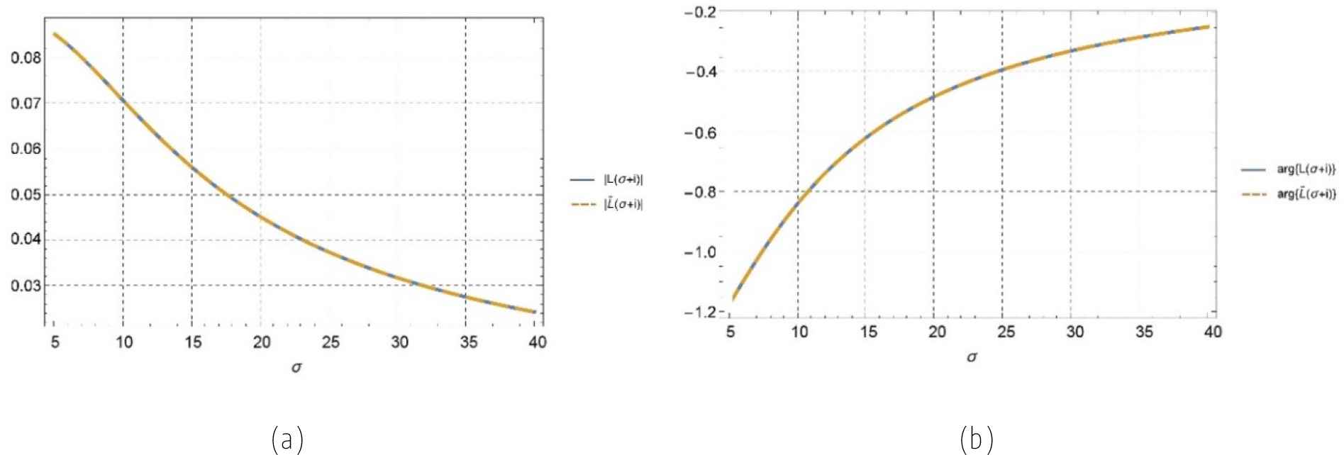
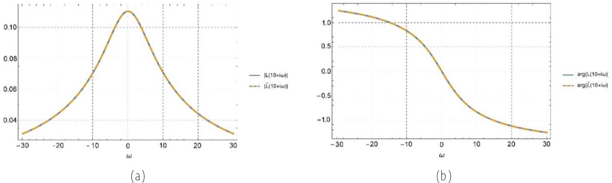
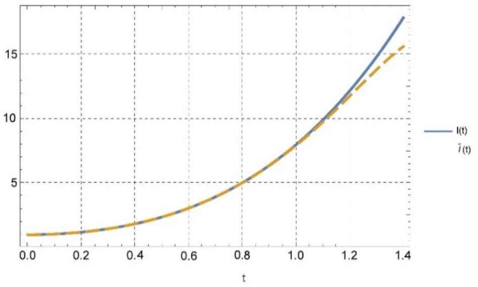
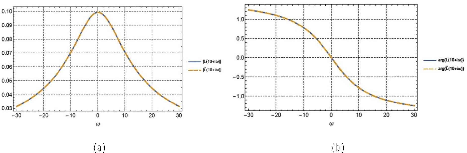
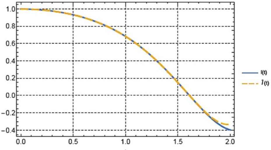
The distributions of $L (s)$ and $\tilde{L} (s)$ along the cut sections $ω = ℑ s = 1$ and $σ = ℜ s = 5$ are reported in Fig. 1 and Fig. 2, respectively. As it can be noticed, the agreement between the exact transform in Eq. (18) (for $ν = π$ ) and the relevant approximation in Eq. (19) is very good especially as $s \to + \infty$ . Conversely, the functions $l (t)$ and $\tilde{l} (t)$ tend to match for $t \to 0^{+}$ as one would expect from theory (see Fig. 3).

5.2.2. Test Case #2

Considering the composed function $J_{ν} (a sinh (t))$ with $ℜ a > 0, ℜ ν > - 1$ , it results [13]:

L (s) = \int_{0}^{+ \infty} J_{ν} (a \sinh (t)) e^{- t s} d t = J_{\frac{ν + s}{2}} (\frac{a}{2}) K_{\frac{ν - s}{2}} (\frac{a}{2}) ℜ s > - \frac{1}{2}

(21)

where

J_{ν}

and

K_{ν}

are Bessel functions. Assuming

ν = 0

and

a = 1

we find the LT:

L (s) = \int_{0}^{+ \infty} J_{0} (\sinh (t)) e^{- t s} d t = J_{\frac{s}{2}} (\frac{1}{2}) K_{- \frac{s}{2}} (\frac{1}{2}) ℜ s > - \frac{1}{2}

(22)

Using our approximation, we have found:

L (s) ≃ \tilde{L} (s) = \int_{0}^{+ \infty} J_{0} (\sinh (t)) e^{- t s} d t = \frac{1}{s} - \frac{1}{2 s^{3}} - \frac{13}{8 s^{5}} - \frac{13}{16 s^{7}} + \frac{9827}{128 s^{9}} + \frac{309649}{256 s^{11}} + O (\frac{1}{s^{13}})

(23)

so that, by inverse Laplace transformation, one can readily conclude that:

\tilde{l} (t) ≃ (1 - \frac{1}{4} t^{2} - \frac{13}{192} t^{4} - \frac{13}{11520} t^{6} + \frac{9827}{5160960} t^{8} + \frac{309649}{928972800} t^{10}) H (t)

(24)

with

H (\cdot)

denoting the classical Heaviside distribution.

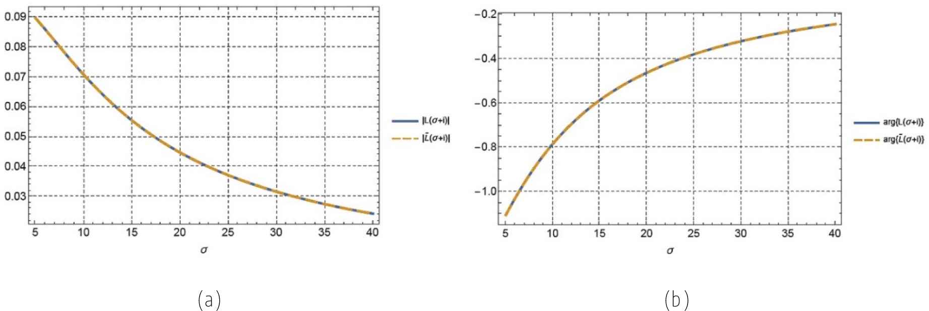
The distributions of $L (s)$ and $\tilde{L} (s)$ along the cut sections $ω = ℑ s = 1$ and $σ = ℜ s = 5$ are reported in Fig. 4 and Fig. 5, respectively. As it can be noticed, the agreement between the exact transform in Eq. (22) and the relevant approximation in Eq. (23) is very good especially as $s \to + \infty$ . Conversely, the functions $l (t)$ and $\tilde{l} (t)$ tend to match for $t \to 0^{+}$ as one would expect from theory (see Fig. 6).

6. AN EXTENSION OF THE BELL POLYNOMIALS

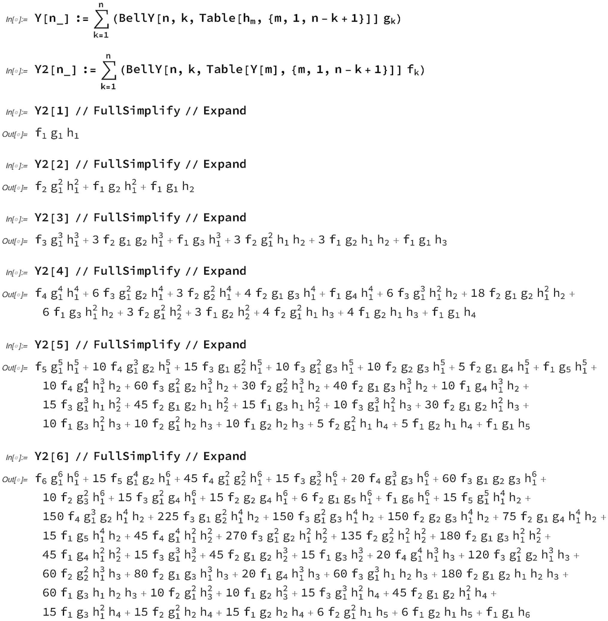
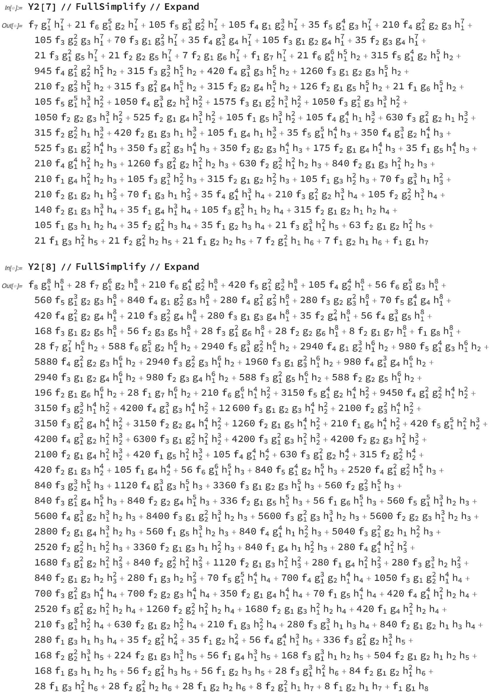
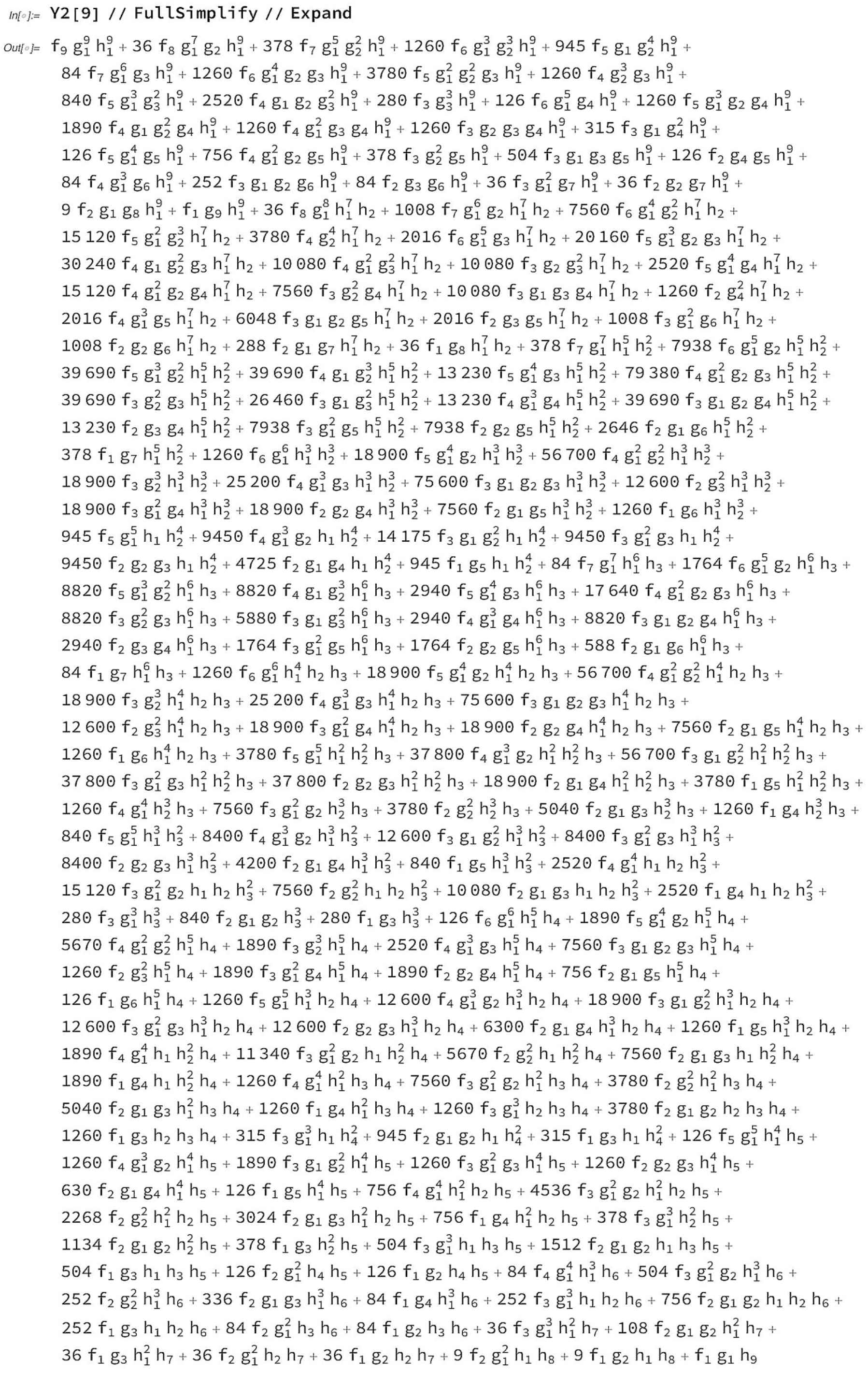
We limit ourselves to the second-order Bell polynomials, $Y_{n}^{[2]} (f_{1}, g_{1}, h_{1}; f_{2}, g_{2}, h_{2}; \dots; f_{n}, g_{n}, h_{n})$ , generated by the $n$ -th derivative of the composed function $Φ (t) : = f (g (h (t)))$ .

Consider the differentiable functions $x = h (t), z = g (x)$ and $y = f (z)$ , and suppose it is possible to use the chain rule for the $n$ -th differentiation of the nested function $Φ (t) : = f (g (h (t)))$ . We use the notations:

Φ_{j} : = D_{t}^{j} Φ (t), f_{h} : = {D_{y}^{h} f (y)|}_{y = g (x)}, g_{k} : = {D_{x}^{k} g (x)|}_{x = h (t)}, h_{r} : = D_{t}^{r} h (t)

(25)

Then the $n$ -th derivative can be represented as:

Φ_{n} = Y_{n}^{[2]} (f_{1}, g_{1}, h_{1}; f_{2}, g_{2}, h_{2}; \dots; f_{n}, g_{n}, h_{n})

where the

Y_{n}^{[2]}

are the second-order Bell polynomials [16].

For example, one has:

\begin{array}{l} Y_{1}^{[2]} (f_{1}, g_{1}, h_{1}) = f_{1} g_{1} h_{1} \\ Y_{2}^{[2]} (f_{1}, g_{1}, h_{1}; f_{2}, g_{2}, h_{2}) = f_{1} g_{1} h_{2} + f_{1} g_{2} h_{1}^{2} + f_{2} g_{1}^{2} h_{1}^{2} \\ Y_{3}^{[2]} (f_{1}, g_{1}, h_{1}; f_{2}, g_{2}, h_{2}; f_{3}, g_{3}, h_{3}) = f_{1} g_{1} h_{3} + f_{1} g_{3} h_{1}^{3} + 3 f_{1} g_{2} h_{1} h_{2} + 3 f_{2} g_{1}^{2} h_{1} h_{2} + 3 f_{2} g_{1} g_{2} h_{1}^{3} + f_{3} g_{1}^{3} h_{1}^{3} \end{array}

The connections with the ordinary Bell polynomials are expressed by the equation:

Y_{n}^{[2]} (f_{1}, g_{1}, h_{1}; \dots; f_{n}, g_{n}, h_{n}) = Y_{n} (f_{1}, Y_{1} (g_{1}, h_{1}); f_{2}, Y_{2} (g_{1}, h_{1}; g_{2}, h_{2}); \dots; f_{n}, Y_{n} (g_{1}, h_{1}; g_{2}, h_{2}; \dots; g_{n}, h_{n}))

Consequently, we deduce the theorem:

Theorem 4.

The following recurrence relation for the second-order Bell polynomials holds true:

\begin{array}{l} Y_{0}^{[2]} = f_{1} \\ Y_{n + 1}^{[2]} (f_{1}, g_{1}, h_{1}; \dots; f_{n + 1}, g_{n + 1}, h_{n + 1}) = \\ \sum_{k = 0}^{n} (\begin{matrix} n \\ k \end{matrix}) Y_{n - k}^{[2]} (f_{2}, g_{1}, h_{1}; f_{3}, g_{2}, h_{2}; \dots; f_{n - k + 1}, g_{n - k}, h_{n - k}) Y_{k + 1} (g_{1}, h_{1}; \dots; g_{k + 1}, h_{k + 1}) \end{array}

The first few second-order Bell polynomials are as follows:

\begin{array}{l} Y_{1}^{[2]} ({[f, g, h]}_{1}) = f_{1} g_{1} h_{1} \\ Y_{2}^{[2]} ({[f, g, h]}_{2}) = f_{1} g_{1} h_{2} + f_{1} g_{2} h_{1}^{2} + f_{2} g_{1}^{2} h_{1}^{2} \\ Y_{3}^{[2]} ({[f, g, h]}_{3}) = f_{1} g_{1} h_{3} + f_{1} g_{3} h_{1}^{3} + 3 f_{1} g_{2} h_{1} h_{2} + 3 f_{2} g_{1} g_{2} h_{1}^{3} + f_{3} g_{1}^{3} h_{1}^{3} \\ Y_{4}^{[2]} ({[f, g, h]}_{4}) = f_{4} g_{1}^{4} h_{1}^{4} + 6 f_{3} g_{1}^{2} g_{2} h_{1}^{4} + 3 f_{2} g_{2}^{2} h_{1}^{4} + 4 f_{2} g_{1} g_{3} h_{1}^{4} + f_{1} g_{4} h_{1}^{4} + 6 f_{3} g_{1}^{3} h_{1}^{2} h_{2} + \\ 18 f_{2} g_{1} g_{2} h_{1}^{2} h_{2} + 6 f_{1} g_{3} h_{1}^{2} h_{2} + 3 f_{2} g_{1}^{2} h_{2}^{2} + 3 f_{1} g_{2} h_{2}^{2} + 4 f_{2} g_{1}^{2} h_{1} h_{3} + 4 f_{1} g_{2} h_{1} h_{3} + f_{1} g_{1} h_{4} \end{array}

(26)

Further values are reported in Appendix II.

7. LAPLACE TRANSFORM OF NESTED FUNCTIONS

Let $f (g (h (t)))$ be a nested function analytic in a neighborhood of the origin, expressed by the Taylor's expansion:

f (g (h (t))) = \sum_{n = 0}^{\infty} a_{n} \frac{t^{n}}{n!}, a_{n} = D_{t}^{n} {[f (g ((h (t)))]}_{t = 0}

(27)

It results:

\begin{array}{l} a_{0} = {\overset{\circ}{f}}_{0} = f (g (h (0)) \\ a_{n} = D_{t}^{n} {[f (g ((h (t)))]}_{t = 0} = Y_{n}^{[2]} (\overset{\circ}{f_{1}}, {\overset{\circ}{g}}_{1}, {\overset{\circ}{h}}_{1}; \dots; {\overset{\circ}{f}}_{n}, {\overset{\circ}{g}}_{n}, {\overset{\circ}{h}}_{n}) (n \geq 1) \end{array}

(28)

where:

\overset{\circ}{f_{h}} : = {D_{x}^{h} f (y)|}_{y = g (0)}, {\overset{\circ}{g}}_{k} : = {D_{t}^{k} g (x)|}_{x = h (0)}, {\overset{\circ}{h}}_{r} : = {D_{t}^{r} h (t)|}_{t = 0}

(29)

Theorem 5.

Consider a nested function $f (g (h (t)))$ which is analytic in a neighborhood of the origin and which can be represented by the Taylor's expansion in Eq. (27). For its LT the following expression holds:

\begin{array}{l} \int_{0}^{+ \infty} f (g ((h (t))) e^{- t s} d t = & \frac{{\overset{\circ}{f}}_{0}}{s} + \sum_{n = 1}^{\infty} Y_{n}^{[2]} ({\overset{\circ}{f}}_{1}, {\overset{\circ}{g}}_{1}, {\overset{\circ}{h}}_{1}; \dots; {\overset{\circ}{f}}_{n}, {\overset{\circ}{g}}_{n}, \overset{\circ}{h}) \frac{t^{n}}{n!} e^{- t s} d t = \\ \frac{{\overset{\circ}{f}}_{0}}{s} + \sum_{n = 1}^{\infty} Y_{n}^{[2]} ({\overset{\circ}{f}}_{1}, {\overset{\circ}{g}}_{1}, {\overset{\circ}{h}}_{1}; \dots; {\overset{\circ}{f}}_{n}, {\overset{\circ}{g}}_{n}, {\overset{\circ}{h}}_{n}) \frac{1}{s^{n + 1}} \end{array}

(30)

Proof.

It is a straightforward application of the definition of second-order Bell's polynomials.

7.1. Example #1

Assuming $f (x) = e^{x - 1}, g (y) = \cos (y), h (t) = sin (t)$ , it results:

\int_{0}^{+ \infty} \exp [cos (\sin (t)) - 1] e^{- t s} d t = \frac{1}{s} - \frac{1}{s^{3}} + \frac{8}{s^{5}} - \frac{127}{s^{7}} + \frac{3523}{s^{9}} - \frac{146964}{s^{11}} + O (\frac{1}{s^{13}})

(31)

The corresponding inverse LT is approximated by:

\tilde{l} (t) ≃ (1 - \frac{1}{2} t^{2} + \frac{1}{3} t^{4} - \frac{127}{720} t^{6} + \frac{3523}{40320} t^{8} - \frac{12247}{302400} t^{10}) H (t)

(32)

with

H (\cdot)

denoting the classical Heaviside distribution.

7.2. Example #2

Assuming $f (x) = log (1 + \frac{x}{2}), g (y) = cosh (y) - 1, h (t) = sin (t)$ , it results:

\int_{0}^{+ \infty} \log [1 + \frac{\cosh (\sin (t)) - 1}{2}] e^{- t s} d t = \frac{1}{2 s^{3}} - \frac{9}{4 s^{5}} - \frac{27}{2 s^{7}} + \frac{1169}{8 s^{9}} - \frac{5869}{2 s^{11}} + O (\frac{1}{s^{13}})

(33)

The corresponding inverse LT is approximated by:

\tilde{l} (t) ≃ (\frac{1}{4} t^{2} - \frac{3}{32} t^{4} + \frac{3}{160} t^{6} - \frac{167}{46080} t^{8} + \frac{5869}{7257600} t^{10}) H (t)

(34)

with

H (\cdot)

denoting the classical Heaviside distribution.

7.3. Example #3

Assuming $f (x) = e^{x}, g (y) = J_{1} (y), h (t) = sin (t)$ , it results:

\begin{array}{l} \int_{0}^{+ \infty} exp [J_{1} (\sin (t))] e^{- t s} d t = \frac{1}{s} - \frac{1}{2 s^{2}} + \frac{1}{4 s^{3}} - \frac{3}{4 s^{4}} - \frac{27}{16 s^{5}} + \frac{77}{32 s^{6}} + \\ \frac{1227}{64 s^{7}} + \frac{385}{128 s^{8}} - \frac{82663}{256 s^{9}} - \frac{439229}{512 s^{10}} + \frac{6754489}{1024 s^{11}} + O (\frac{1}{s^{12}}) \end{array}

(35)

The corresponding inverse LT is approximated by:

\begin{array}{l} \tilde{l} (t) ≃ (1 + \frac{1}{2} t + \frac{1}{8} t^{2} - \frac{1}{8} t^{3} - \frac{9}{128} t^{4} + \frac{77}{3840} t^{5} + \frac{409}{15360} t^{6} + \frac{11}{18432} t^{7} - \\ \frac{11809}{1474560} t^{8} - \frac{62747}{26542080} t^{9} + \frac{964927}{530841600} t^{10}) H (t) \end{array}

(36)

with

H (\cdot)

denoting the classical Heaviside distribution.

7.4. Example #4

Assuming $f (x) = \arctan (x), g (y) = y^{\frac{1}{3}}, h (t) = cosh (t)$ , it results:

\int_{0}^{+ \infty} \arctan [{(cosh (t))}^{\frac{1}{3}}] e^{- t s} d t = \frac{π}{4 s} + \frac{1}{6 s^{3}} - \frac{1}{3 s^{5}} + \frac{43}{18 s^{7}} - \frac{338}{9 s^{9}} + \frac{18523}{18 s^{11}} + O (\frac{1}{s^{13}})

(37)

The corresponding inverse LT is approximated by:

\tilde{l} (t) ≃ (\frac{π}{4} + \frac{1}{12} t^{2} - \frac{1}{72} t^{4} + \frac{43}{12960} t^{6} - \frac{169}{181440} t^{8} + \frac{18523}{65318400} t^{10}) H (t)

(38)

with

H (\cdot)

denoting the classical Heaviside distribution.

Remark 6:

Note also that successive Bell polynomials are represented exclusively by sums, products and powers, avoiding operations that may generate numerical instability. The use of computers allows calculations to be performed stably and quickly, even though the number of products to be added increases rapidly with the number n. In our calculations it was possible to obtain a sufficient approximation by limiting ourselves to order n = 10.

8. CONCLUSION

We have presented a method for approximating the integral of analytic composed functions. Considering the Taylor expansion of the given function and representing their coefficients in terms of Bell’s polynomials, the integral reduces to the computation of an approximating series, which obviously converges if the integral is convergent. This methodology has been applied to the LT of an analytic composed function, starting from the case of analytic nested exponential functions, based on the complete Bell polynomials, computed by using the program Mathematica^®, and shown in Appendix I.

In the second part the LT of analytic nested functions is considered, and the second-order Bell’s polynomials used in this approach are reported in Appendix II. We want to stress that, even if we dealt with a basic subject, we have not found in the literature any general method for approximating this type of LTs, a gap which, in our opinion, has been now filled up. A graphical verification of the proposed technique, performed in the case when both the analytical forms of the transform and anti-transform are known, proved the correctness of our results.

The method used in this article has also been applied in other cases such as:

•
the LT of analytic composed functions of several variables [17,18];
•
the LT of composed functions of two variables, making use of Bell’s polynomials in two dimensions introduced and studied in a previous article [19,20];
•
the sine and cosine Fourier transform of particular nested functions [21].

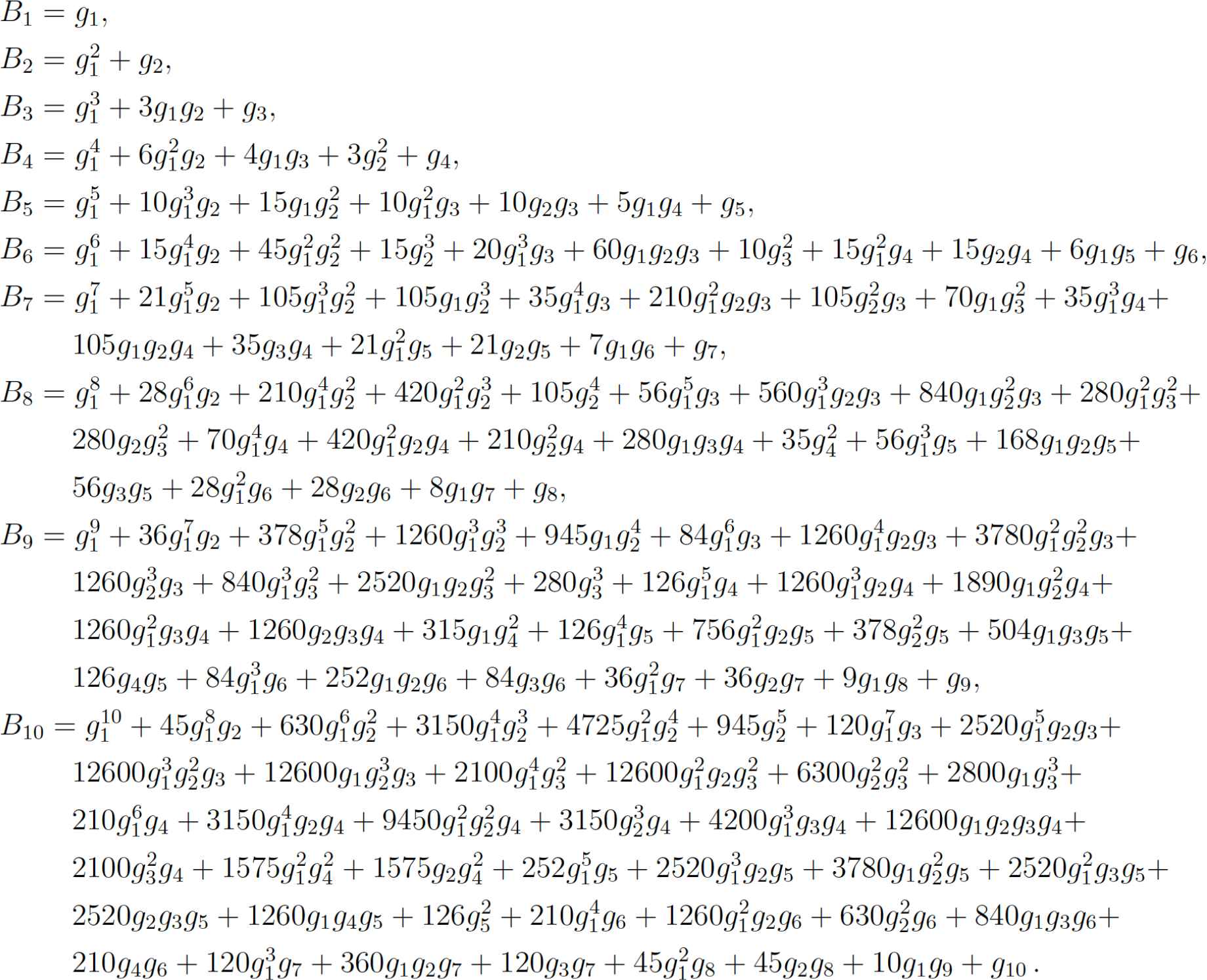
APPENDIX I: TABLE OF COMPLETE BELL POLYNOMIALS

APPENDIX II: TABLE OF SECOND-ORDER BELL POLYNOMIALS

REFERENCES

[1]

E.T. Bell. Exponential Polynomials. Annals of Mathematics, 1934, 35(2): 258–277. https://doi.org/10.2307/1968431

[2]

J. Riordan. An Introduction to Combinatorial Analysis. Chichester: John Wiley & Sons, 1958.

[3]

P. Natalini, P.E. Ricci. Bell Polynomials and Modified Bessel Functions of Half-Integral Order. Applied Mathematics and Computation, 2015, 268: 270–274. https://doi.org/10.1016/j.amc.2015.06.069

[4]

R. Orozco López. Solution of the Differential Equation y^(k) = e^ay, Special Values of Bell Polynomials, and (k,a)-Autonomous Coefficients. Journal of Integer Sequences, 2021, 24(8): 21.8.6.

[5]

F. Qi, D.-W. Niu, D. Lim, Y.-H. Yao. Special Values of the Bell Polynomials of the Second Kind for Some Sequences and Functions. Journal of Mathematical Analysis and Applications, 2020, 491(2): 124382. https://doi.org/10.1016/j.jmaa.2020.124382

[6]

P.E. Ricci, P. Natalini. Bell Polynomials and 2nd Kind Hypergeometric Bernoulli Numbers. Seminar of I. Vekua Institute of Applied Mathematics, 2022, 48: 36–45.

[7]

P.E. Ricci. Bell Polynomials and Generalized Laplace Transforms. Integral Transforms and Special Functions, 2022, 33(12): 966–977. https://doi.org/10.1080/10652469.2022.2059077

[8]

P. Natalini, P.E. Ricci. Higher Order Bell Polynomials and the Relevant Integer Sequences. Applicable Analysis and Discrete Mathematics, 2017, 11(2): 327–339. https://doi.org/10.2298/AADM1702327N

[9]

S.M. Roman. The Formula of Faà di Bruno. The American Mathematical Monthly, 1980, 87(10): 805–809. https://doi.org/10.1080/00029890.1980.11995156

[10]

S.M. Roman, G.-C. Rota. The Umbral Calculus. Advances in Mathematics, 1978, 27(2): 95–188. https://doi.org/10.1016/0001-8708(78)90087-7

[11]

G.H. Hardy, S. Ramanujan. Asymptotic Formulae in Combinatory Analysis. Proceedings of the London Mathematical Society, 1918, s2-17(1): 75–115. https://doi.org/10.1112/plms/s2-17.1.75

[12]

A. Ghizzetti, A. Ossicini. Trasformate di Laplace e Calcolo Simbolico. Turin: Unione Tipografico-Editrice Torinese (UTET), 1971. (in Italian)

[13]

F. Oberhettinger, L. Badii. Tables of Laplace Transforms. Heidelberg: Springer-Verlag, 1973. https://doi.org/10.1007/978-3-642-65645-3

[14]

L. Amerio. Funzioni Analitiche e Trasformazione di Laplace. Milan: Tamburini, 1976. (in Italian)

[15]

A. Erdélyi, W. Magnus, F. Oberhettinger, F.G. Tricomi. Higher Transcendental Functions, Vol. II. New York: McGraw-Hill Book Company, 1953.

[16]

P. Natalini, P.E. Ricci. An Extension of the Bell Polynomials. Computers & Mathematics With Applications, 2004, 47(4–5): 719–725. https://doi.org/10.1016/S0898-1221(04)90059-4

[17]

A. Bernardini, P. Natalini, P.E. Ricci. Multidimensional Bell Polynomials of Higher Order. Computers & Mathematics With Applications, 2005, 50(10–12): 1697–1708. https://doi.org/10.1016/j.camwa.2005.05.008

[18]

D. Caratelli, P.E. Ricci. Bell’s Polynomials and Laplace Transform of Higher Order Nested Functions. Symmetry, 2022, 14(10): 2139. https://doi.org/10.3390/sym14102139

[19]

D. Caratelli, R. Srivastava, P.E. Ricci. The Laplace Transform of Composed Functions and Bivariate Bell Polynomials. Axioms, 2022, 11(11): 591. https://doi.org/10.3390/axioms11110591

[20]

S. Noschese, P.E. Ricci. Differentiation of Multivariable Composite Functions and Bell Polynomials. Journal of Computational Analysis and Applications, 2003, 5(3): 333–340. https://doi.org/10.1023/A:1023227705558

[21]

D. Caratelli, P.E. Ricci. On a Set of Sine and Cosine Fourier Transforms of Nested Functions. Dolomites Research Notes on Approximation, 2022, 15(1): 11–19. https://doi.org/10.14658/PUPJ-DRNA-2022-1-2

Previous Article In Volume

Next Article In Volume

Cite This Article

ris

TY  - CONF
AU  - Paolo Emilio Ricci
AU  - Diego Caratelli
AU  - Sandra Pinelas
PY  - 2023
DA  - 2023/11/29
TI  - Laplace Transform Approximation of Nested Functions Using Bell’s Polynomials
BT  - Proceedings of the 1st International Symposium on Square Bamboos and the Geometree (ISSBG 2022)
PB  - Athena Publishing
SP  - 55
EP  - 70
SN  - 2949-9429
UR  - https://doi.org/10.55060/s.atmps.231115.006
DO  - https://doi.org/10.55060/s.atmps.231115.006
ID  - Ricci2023
ER  -

copy

enw

bib

Article Contents

Proceedings of the 1st International Symposium on Square Bamboos and the Geometree (ISSBG 2022)

1. INTRODUCTION

2. RECALLING THE BELL POLYNOMIALS

Remark 1:

3. RECALLING THE LAPLACE TRANSFORM

Remark 2:

3.1. Main Properties and an Example

4. LAPLACE TRANSFORM OF COMPOSED FUNCTIONS

Theorem 3.

Proof.

5. THE CASE OF THE EXPONENTIAL FUNCTION

5.1. First Examples

5.2. Graphical Display in Two Known Cases

5.2.1. Test Case #1

5.2.2. Test Case #2

6. AN EXTENSION OF THE BELL POLYNOMIALS

Theorem 4.

7. LAPLACE TRANSFORM OF NESTED FUNCTIONS

Theorem 5.

Proof.

7.1. Example #1

7.2. Example #2

7.3. Example #3

7.4. Example #4

Remark 6:

8. CONCLUSION

APPENDIX I: TABLE OF COMPLETE BELL POLYNOMIALS

APPENDIX II: TABLE OF SECOND-ORDER BELL POLYNOMIALS

REFERENCES

Cite This Article