
Revised 16 July 2023
Accepted 29 September 2023
Available Online 29 November 2023
- DOI
- https://doi.org/10.55060/s.atmps.231115.007
- Keywords
- Mixed differential equations
Delays and advances
Stability of solutions - Abstract
Mixed differential equations with advance and delay occur in many problems in economy, biology, physics and engineering. The concept of delay is related to the memory of systems, where past events influence current behavior. The concept of advance is related to potential future events which are known at the current time, and which could be useful for decision making. In this article various examples are given of difference and differential equations, classical, with delay, and with delay and advances (the mixed ones). It is well known that the solutions of these types of equations cannot be obtained in closed form. It is not quite clear how to formulate an initial value problem for such equations and the existence and uniqueness of solutions becomes a complicated issue. To study the oscillation of solutions of differential equations, we need to assume that there exists a solution of such equations on the half line.
- Copyright
- © 2023 The Authors. Published by Athena International Publishing B.V.
- Open Access
- This is an open access article distributed under the CC BY-NC 4.0 license (https://creativecommons.org/licenses/by-nc/4.0/).
1. DIFFERENCE AND DIFFERENTIAL EQUATIONS
1.1. Tumor Growth Cancer Model
In [1], the authors consider the following system where
- •
- •
- •
- •
- •
- •
- •
- •
- •
- •
The equilibrium points of the system shown in Eq. (1) are:
The equilibrium point
Example 1.
For the system shown in Eq. (1) with:
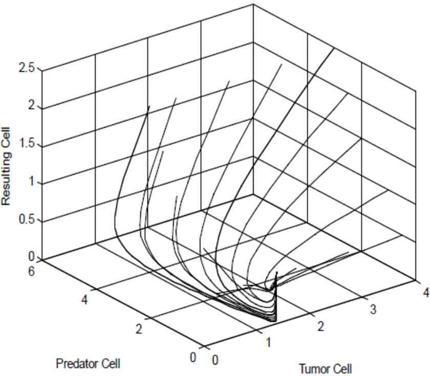
The equilibrium point
1.2. Biolarvicides Against Malaria Model
Biolarvicides are in use in several parts of the world for malaria vector control (see [2]). Consider the system:
- •
- •
- •
- •
- •
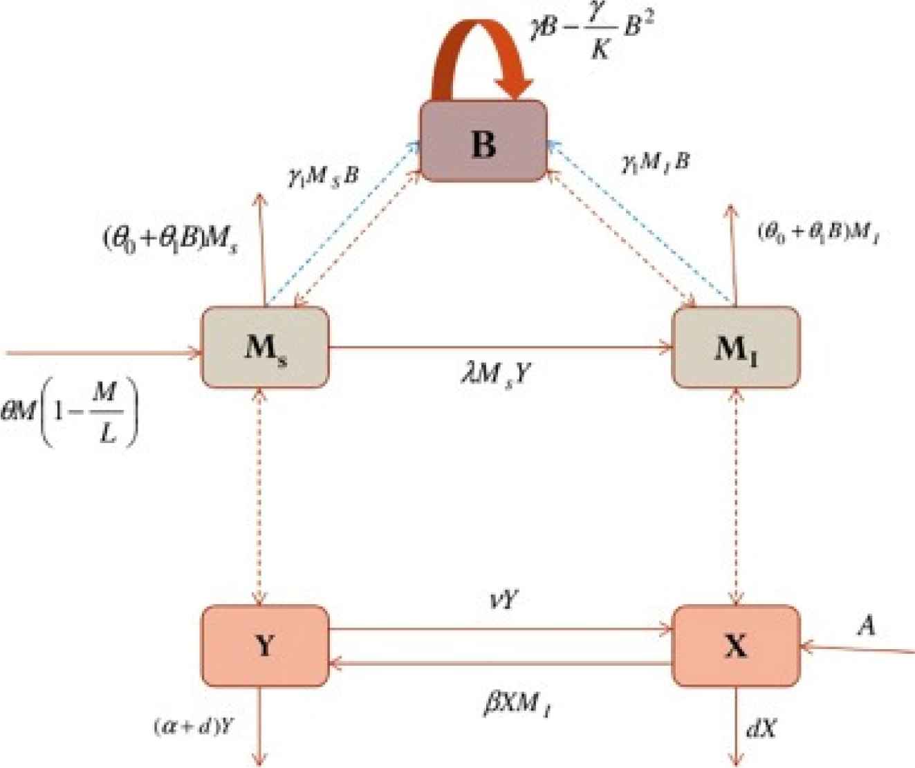
Schematic overview of the system. The direction of each solid line represents movement of population along that line within the same species. The bi-directional dotted lines between boxes indicate a mass-action interaction. The single directional dotted line indicates increase of bacteria population (for example,
The equilibrium points of the system shown in Eq. (2) are:
- •
- •
- •
- •
- •
- •
2. DIFFERENCE AND DIFFERENTIAL EQUATIONS WITH DELAYS
2.1. Logistic Equations With Delays
Population density is unlikely to elicit an instant response to the per capita growth rate.
For example, the effect of food scarcity available to young immatures can only be felt later when they reach maturity expressing lower fertility rates. By designating τ the delay interval we get the delayed logistic equation:
The earliest delay model in mathematical biology is Hutchinson's equation in 1948 [3], when he modified the classical logistic equation, with a delay term to incorporate hatching and maturation periods into the model and account for oscillations, in the population of Daphnia. Such oscillations (Fig. 3) are in part due to the fact that the fertility of a parthenogenic female is determined, not merely by the population density at a given time, but also by the past densities to which it has been exposed [4].
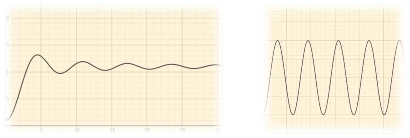
Oscillations.
2.2. Survival of Blood Cells
The delay differential equation:
- •
- •
- •

Red blood cells.
The delay differential equation:
The positive equilibrium point is given by:
The solutions oscillate about
2.3. Infinite Impulse Response Filter
A filter is a system that functions to extract the data from noise in a signal:
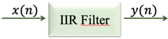
The defining equation for an IIR filter is the difference equation:
- •
- •
- •
In [6] it is shown that this equation is equivalent to the difference equation:
3. DIFFERENCE AND DIFFERENTIAL EQUATIONS WITH DELAYS AND ADVANCES
Mixed differential equations have mixed arguments, with delay and advance (Fig. 5). They occur in many problems in economy, biology, physics and engineering. However, this class of equations has been much less studied than other classes of functional differential equations.

Mixed type equations allow to establish conditions between past and potential future events to get a good decision.
Why are these types of equations a challenge? It is well known that the solutions of these types of equations cannot be obtained in closed form [7]. It is not clear how to formulate an initial value problem for such equations and the existence and uniqueness of solutions becomes complicated [8]. To study the oscillation of solutions of differential equations, we need to assume that there exists a solution of such equations on the half line.
Example 2.
[9] Let the initial value problem with
With
Then:
Example 3.
[9] For
Remark:
Note that for the delayed argument
An example with nerve conduction was studied in [10].
The equation:
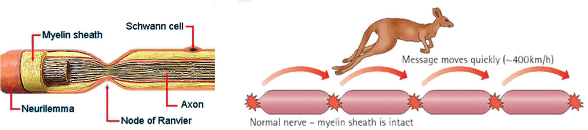
Nerve, consisting of axon, myelin sheath and nodes of Ranvier.
In the equation:
The constant r is unknown a priori and must be found simultaneously with
Using the Ohm Law and the Taylor expansion around 0 the equation:
Using numerical methods, we obtain the solutions in Fig. 7.
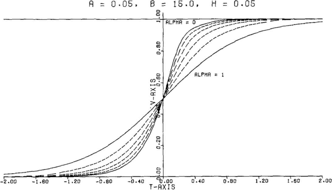
Graph of solutions changes when approaching target problem from test problem.
This means the rise time of the membrane potential is faster for lower threshold potential.
Example 4.
The linear autonomous mixed type differential equation:
Example 5.
Stability and determinacy conditions for linear mixed type functional differential equations were studied in [13]:
In this study, the necessary conditions for the existence, uniqueness and stability of a solution to mixed type functional equations were obtained.
4. STABILITY AND SOLUTIONS IN DIFFERENTIAL EQUATIONS WITH DELAYS AND ADVANCES
Consider the differential equation of mixed type:
- •
- •
We define:
We specify an initial condition of the form:
By a solution of:
If a solution of:
The solution of:
Otherwise, the solution is said to be unstable.
The solution is called asymptotically stable if it is stable in the above sense and in addition there exists a number
5. ESTIMATION OF SOLUTIONS AND STABILITY CRITERIA
Theorem 1.
[14] Let
Then the solution
Moreover, the solution is:
- •
stable if
- •
asymptotically stable if
- •
unstable if
An important Lemma is the following.
Lemma 1.
[14] Assume that:
Then, in the interval
Corollary 1.
[14] Assume that:
Then the solution of:
- •
asymptotically stable if
- •
unstable if
Example 6.
[14] Consider the equation:
Notice that in this case we have:
The characteristic equation is:
So,
The function
The only one root of
Then, for
So, the solution is asymptotically stable.
In this example, stability analysis can be performed using Corollary 1 of Lemma 1 without using the characteristic equation. Indeed, we get:
Thus, according to Lemma 1, it states that a real root must pass in the interval (−2, 2).
Finally, from Corollary 1 we obtain:
Example 7.
Consider the equation:
Here
So,
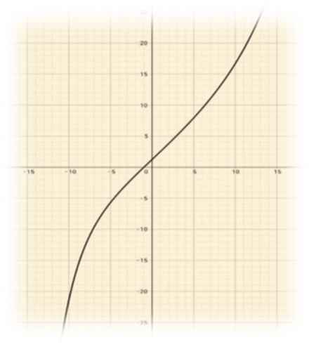
The graph of the function
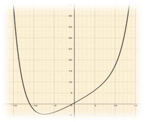
The function
Let
So for
Let
Then for
ACKNOWLEDGMENT
Supported by the Center for Research and Development in Mathematics and Applications (CIDMA) through the Portuguese Foundation for Science and Technology (FCT – Fundação Para a Ciência e a Tecnologia), references UIDB/04106/2020 and UIDP/04106/2020.
REFERENCES
Cite This Article
TY  - CONF
AU  - Sandra Pinelas
PY  - 2023
DA  - 2023/11/29
TI  - Stability of Solutions in Mixed Differential Equations
BT  - Proceedings of the 1st International Symposium on Square Bamboos and the Geometree (ISSBG 2022)
PB  - Athena Publishing
SP  - 71
EP  - 83
SN  - 2949-9429
UR  - https://doi.org/10.55060/s.atmps.231115.007
DO  - https://doi.org/10.55060/s.atmps.231115.007
ID  - Pinelas2023
ER  -


